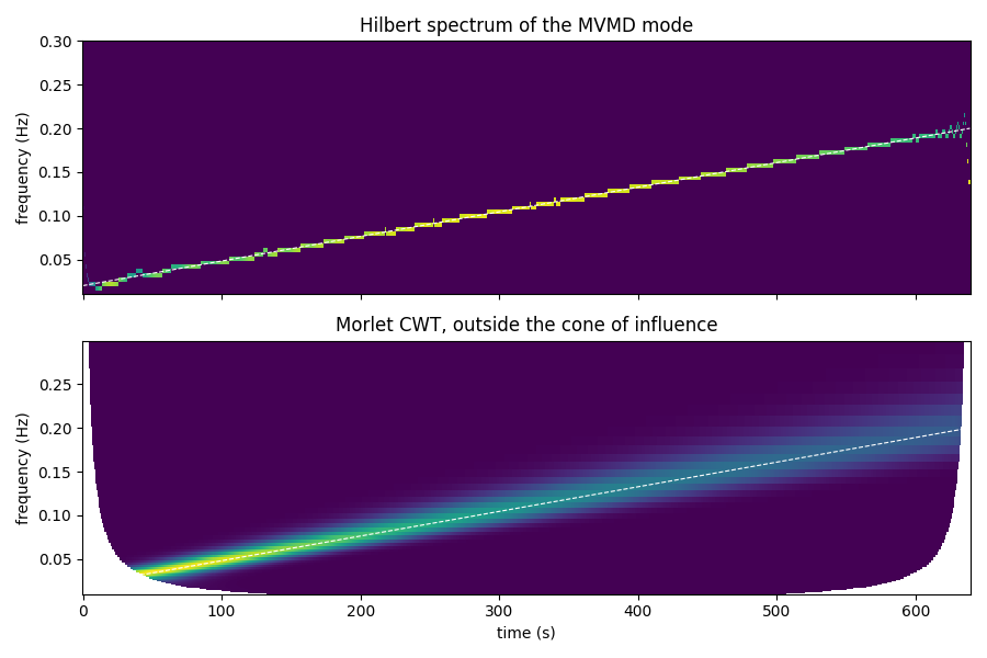
Hilbert spectrum and Morlet wavelets on a chirp

A tone that sweeps from 0.02 to 0.2 Hz. The Hilbert spectrum of its MVMD modes follows the sweep sample by sample; the Morlet CWT smooths it over each wavelet’s length and marks where edge effects make values unreliable (the cone of influence).

import matplotlib.pyplot as plt
import numpy as np

import modewise

fs = 1.25
t = np.arange(800) / fs
phase = 2 * np.pi * (0.02 * t + 0.5 * (0.18 / t[-1]) * t**2)
x = np.vstack([np.sin(phase)])

modes = modewise.mvmd(x, fs, num_modes=1, alpha=50.0)
hilbert = modewise.hilbert_spectrum(modewise.hilbert(modes), 0.01, 0.3, 60)
cwt = modewise.cwt(x, fs, 0.01, 0.3, 60)

fig, (a, b) = plt.subplots(2, 1, figsize=(9, 6), sharex=True)
a.pcolormesh(t, hilbert.frequencies_hz, hilbert.power[0], shading="auto")
a.set_title("Hilbert spectrum of the MVMD mode")
b.pcolormesh(t, cwt.frequencies_hz, np.where(cwt.reliable, cwt.power[0], np.nan), shading="auto")
b.set_title("Morlet CWT, outside the cone of influence")
for ax in (a, b):
    ax.plot(t, 0.02 + (0.18 / t[-1]) * t, "w--", lw=0.8)
    ax.set_ylabel("frequency (Hz)")
b.set_xlabel("time (s)")
fig.tight_layout()