Three ways to split a signal into modes

A slow (0.02 Hz) and a fast (0.18 Hz) rhythm on a drift, decomposed by MVMD, EMD and the MODWT multiresolution analysis.

• MVMD finds the number of modes you ask for, at frequencies it adapts to the data.

• EMD finds as many oscillations as the data hold, with the drift as its residual (mode 0). It also pulls two weak slow modes out of the drift and the edges, a known EMD behaviour.

• The MODWT splits into fixed octaves. The 0.02 Hz tone sits at the edge between two octaves at this sampling rate, so the smooth and D5 share it.

EMD and the MODWT add back up to the signal exactly; MVMD with tau = 0 leaves out what does not fit its modes.

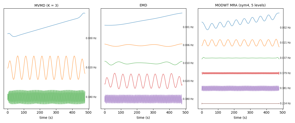
MVMD (K = 3): 3 modes, largest reconstruction error 2.68e-01
EMD: 5 modes, largest reconstruction error 4.44e-16
MODWT MRA (sym4, 5 levels): 6 modes, largest reconstruction error 2.69e-12

import matplotlib.pyplot as plt
import numpy as np

import modewise

fs = 1.25
t = np.arange(600) / fs
x = np.vstack([np.sin(2 * np.pi * 0.02 * t) + 0.6 * np.sin(2 * np.pi * 0.18 * t) + 0.004 * t])

results = {
    "MVMD (K = 3)": modewise.mvmd(x, fs, num_modes=3, alpha=2000.0, init="linear", tau=0.0),
    "EMD": modewise.emd(x, fs),
    "MODWT MRA (sym4, 5 levels)": modewise.modwt_mra(x, fs, levels=5, boundary="reflection"),
}

fig, axes = plt.subplots(1, 3, figsize=(12, 5), sharex=True)
for ax, (name, d) in zip(axes, results.items()):
    for k in range(d.n_modes):
        ax.plot(t, d.modes[k, 0] - 2.5 * k, lw=0.8)
        ax.text(t[-1] + 5, -2.5 * k, f"{d.centre_frequencies_hz[k]:.3f} Hz", va="center", fontsize=7)
    ax.set_title(name, fontsize=10)
    ax.set_yticks([])
    ax.set_xlabel("time (s)")
fig.tight_layout()

for name, d in results.items():
    error = np.abs(d.modes.sum(axis=0) - x).max()
    print(f"{name}: {d.n_modes} modes, largest reconstruction error {error:.2e}")